Section 4 Mapping an invasive species with object-based image analysis
For running this example you have to download the zip file in the
following link. Then uncompress the file and
remember to keep the file names and folder structure intact.
We will also need Orfeo Toolbox (OTB) to run this example since Large
Scale Mean Shift image segmentation algorithm will be used. To install
it go to this link (check
also the installation section).
4.1 Introduction
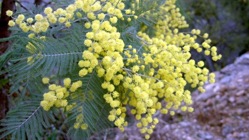
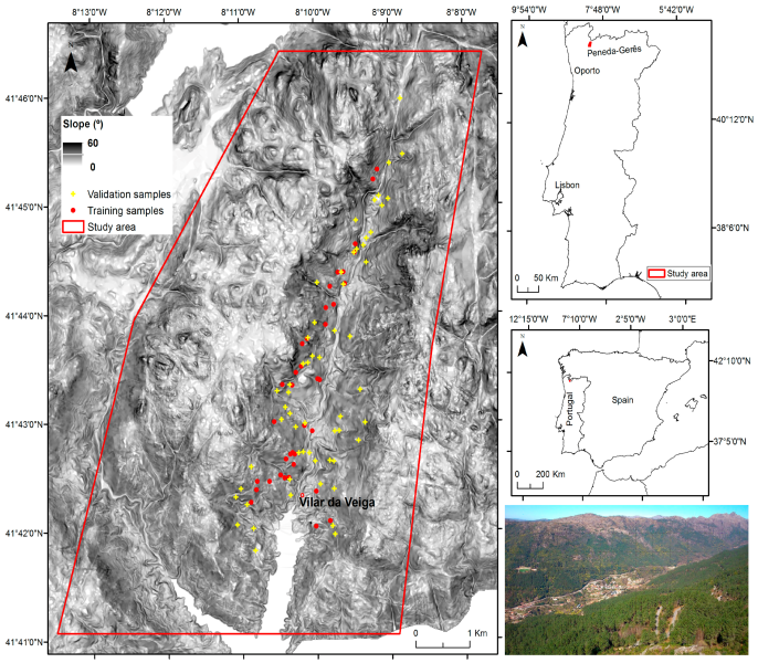
In this example we are going to map areas invaded by Acacia dealbata in Vilar da Veiga, a mountainous area located in Peneda-Geres National Park, NW Portugal. Total precipitation amounts to 1300 mm/year and mean annual temperature to 13 ºC, with large amplitude in mean annual values between cold and warm seasons (-10 to 35 ºC). Elevation ranges from 145 to 1253m with steep slopes.
Scrub and deciduous oak forests developed on granite bedrock and are the main vegetation types, as a follow-up of the abandonment of extensive husbandry. Pine forests are also another relevant vegetation type, especially on common land. Agricultural areas occupy a small and decreasing extent at lower altitudes.
A. dealbata was locally introduced by forestry services to stabilize slopes around the start of the XXth century. However, due to management practices, abandonment and wildfires in the region, it has become widespread throughout the landscape.
4.2 Workflow & data
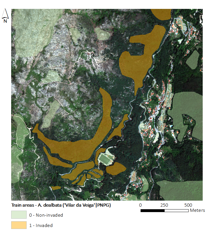
To map the actual distribution of A. dealbata, we will use one WorldView-2 (WV2) image (with eight spectral bands) and training data (i.e., hand-digitized patches delineated using the WV2 image and after field visits to the site). These data contains both invaded and non-invaded patches.
The figure below presents a RGB composite of the WV2 image with training areas overlapped.
4.2.1 Input image data
The Worldview-2 (WV2) image tat we are going to use was collected during summer (23 June 2013). WV2 platform records data in eight spectral bands with a ground resolution of 2 m:
- [B1] Coastal blue (400 - 450nm),
- [B2] Blue (450 - 510nm),
- [B3] Green (510 - 580nm),
- [B4] Yellow (590 - 630nm),
- [B5] Red (630 - 690nm),
- [B6] Red edge (710 - 750nm),
- [B7] Near-Infrared 1 (770 - 900nm), and
- [B8] Near Infrared 2 (860 - 1040nm).
Imagery pre-processing consisted in the orthorectification of the scene using a Digital Elevation Model (DEM; 20 m spatial resolution) and a bilinear convolution algorithm based on six ground control points, yielding average Root Mean Square Error values (RMSE) of 1.45 m. Surface reflectance was obtained by further processing the data with atmospheric correction.
4.2.2 Object-based Image Analysis (OBIA) workflow
An Object-based Image Analysis (OBIA) approach will be employed in this exercise. The workflow is presented in the figure below.
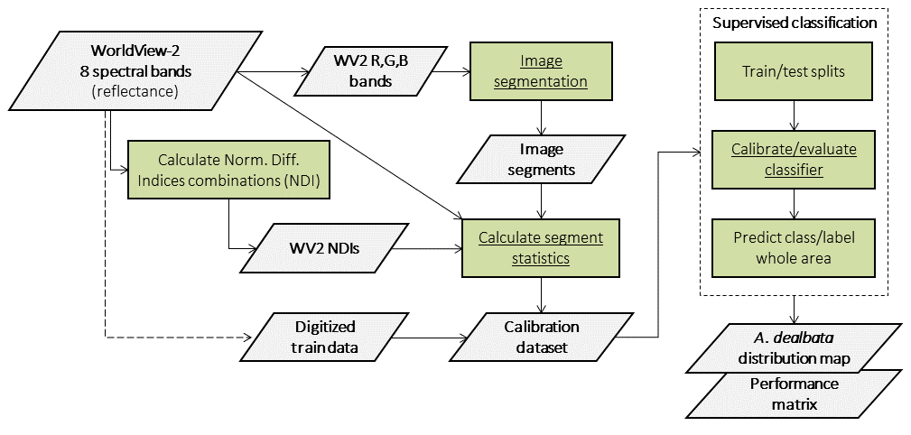
To map the target species we will use SegOptim - a R package used to perform object-based analyses of EO data. SegOptim allows to interface multiple GIS/RS analysis software, such as Orfeo Toolbox (OTB), GRASS, SAGA, etc. and use them to perform image segmentation.
Using the segmented image, we can then run supervised classification, which allows combining field or digitized training data with spectral image features to obtain maps with the distribution of target species or land cover types. SegOptim uses three main input layers described in the figure below.
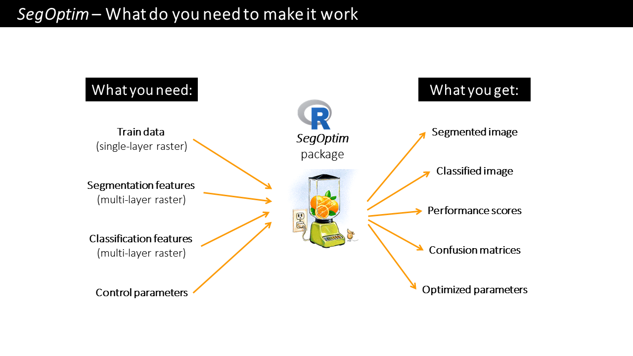
A brief description of SegOptim package inputs:
Training data: typically a single-layer
SpatRaster(fromterrapackage) containing samples for training a classifier. The input format can be of any type included in theterrapackage.Segmentation features: typically a multi-layer
SpatRasterwith features used only for the segmentation stage (e.g., spectral bands, spectral indices, texture). This data will be used by the segmentation algorithm to group similar neighboring pixels into objects (or ‘super-pixels’ or regions).Classification features: also a multi-layer
SpatRasterwith features used for classification (e.g., spectral bands and indices, texture, elevation, slope). The input format can be of any type included in theterra. This will allow the classification algorithm to extract/learn the spectral profile and train the classification functions/rules.
Use R help system to get more info on SegOptim functions.
4.3 Inputs
Change the working directory to the folder where the test data is (download at link and uncompress the zip file if you have not done that yet). Test data has three directories containing segmentation and classification features, as well as train data.
The following paths define inputs required to run SegOptim as well as
outputs. You also need to define the path to the OTB binaries folder
(variable: otbPath, check below).
library(terra)
library(randomForest)
library(SegOptim)

# Change this!!!
setwd("D:/MyDocs/R-dev/SegOptim_Tutorial/data")

# Path to raster data used for image segmentation
# In SEGM_FEAT directory
inputSegFeat.path <- "./SEGM_FEAT/SegmFeat_WV2_b532.tif"

# Path to training raster data
# [0] Non-invaded areas [1] Acacia dealbata invaded areas
# In TRAIN_AREAS directory
trainData.path <- "./TRAIN_AREAS/TrainAreas.tif"

# Path to raster data used as classification features
# In CLASSIF_FEAT directory
classificationFeatures.path <- c("./CLASSIF_FEAT/ClassifFeat_WV2_NDIs.tif",
                                 "./CLASSIF_FEAT/ClassifFeat_WV2_SpectralBands.tif")

# Path to Orfeo Toolbox binaries
otbPath <- "C:/OTB/bin"

# Check if the files and folders exist!
if(!file.exists(inputSegFeat.path))
  print("Could not find data for image segmentation!")

if(!file.exists(trainData.path))
  print("Could not find training data!")

if(!(file.exists(classificationFeatures.path[1]) | file.exists(classificationFeatures.path[2])))
  print("Could not find data for classification!")

if(!dir.exists(otbPath))
  print("Could not find Orfeo Toolbox binaries!")
If you receive a message from the above code chunk you have to correct your data paths.
4.5 Run OTB image segmentation
This section will use SegOptim interface functions to run OTB’s Large Scale Mean Shift (LSMS) image segmentation algorithm. Segmentation involves the partitioning of an image into a set of jointly exhaustive and mutually disjoint regions (a.k.a. segments, composed by multiple image pixels), that are internally more homogeneous and similar, compared to adjacent ones. Image segments are then related to geographic objects of interest (e.g., forests, agricultural or urban areas) through some form of object-based classification (the following step in this exercise).
Mean shift algorithm was firstly proposed by Fukunaga and Hostetler (1975) as a non-parametric density estimation algorithm that converges rapidly on the local maximum of a probability density function through iterations. It was successfully applied to image segmentation by Comaniciu and Meer (1999), with the advantage of not requiring prior knowledge of the number of clusters and not constraining the shape of the clusters. The implementation in OTB, extends the mean-shift algorithm so it can handle large images. Go to: link for more details on mean-shift or read the paper on LSMS:
Michel, J. et al. (2015). Stable Mean-Shift Algorithm and Its Application to the Segmentation of Arbitrarily Large Remote Sensing Images. IEEE Transactions on Geoscience and Remote Sensing (53-2:952-964).
## To know more about the algorithm and its parameters use the help
?segmentation_OTB_LSMS

## Run the segmentation
outSegmRst <- segmentation_OTB_LSMS(
                      # Input raster with features/bands to segment
                      inputRstPath = inputSegFeat.path,
                      # Algorithm params
                      SpectralRange = 3.1,
                      SpatialRange = 4.5,
                      MinSize = 21,
                      # Output
                      outputSegmRst = outSegmRst.path,
                      verbose = TRUE,
                      otbBinPath = otbPath,
                      lsms_maxiter = 50)

# Check the file paths with outputs
print(outSegmRst)

# Load the segmented raster and plot it
segmRst <- rast(outSegmRst$segm)

plot(segmRst)
You can use a GIS software to better inspect and visualize the output segmented raster. Notice that each segment is indexed by an integer number.
NOTE:
Image segmentation parameters need proper tuning to obtain the best
results out of object-based analyses. This requires testing different
parametrizations and values to find which values fit the best to each
case. SegOptim (as the name suggests) allows to optimize these
parameters! However, that is the subject of other section ;-)
4.6 Load train data and classification features
This code chunk is used to load train data and classification features. Train data for SegOptim is simply a raster file with digitized training cases. These are later imported into image segments as we will see. In our case, the file contains areas invaded by A. dealbata (1’s) and non-invaded (0’s).
As for classification features, the files contain:
- Surface reflectance for the eight WV2 bands;
- All combinations (without order) of Normalized Difference Indices (NDI; 28 in total), calculated as:
\[NDI = \frac{(b_i - b_j)}{(b_i + b_j)}\]
Where \(b_i\) and \(b_j\) are any two different spectral bands. In total we
will use 36 features (or variables) for supervised classification. Run
the following code chunk to load the data using terra package
functionalities.
4.7 Prepare the calibration dataset
In this step we will assemble the training data required to the supervised classification. This will import training data into each image segment (via a threshold rule). In this case, segments that are covered in 50% or more by the training pixels will be considered as valid cases either for 0’s (non-invaded) or 1’s (invaded).
We will also use this functions to calculate some statistics from the classification features raster. This will aggregate pixel values in each segment through the average function (other aggregation measures can be used; e.g. std.-dev., median, quantiles, skewness, kurtosis).
Using this function will produce an object of class SOptim.CalData containing two elements:
calData - A data frame object containing calibration data for training and evaluating a classifier algorithm. The first column (named “SID”) contains the ID of each segment, and the second column (named “train”) holds the segment class (or label). The following n columns hold the classification features for training;
classifFeatData - A data frame containing all segments and features from inputs. The first column (named “SID”) holds the unique identifier for each image segment. The following n columns are used as classification features. Typically this dataset is used for predicting the target class after calibrating a certain classifier algorithm.
Run the following code chunk to generate the calibration dataset.
4.8 Calibrate/evaluate the supervised classifier
We will use the training data in combination with satellite data (NDIs and original spectral bands) to map the distribution of A. dealbata. The Random Forest (RF) algorithm will be used for this purpose. RF are an ensemble learning method for classification, regression and other tasks, that operate by constructing multiple decision trees during the training stage and outputting the class that is the mode of the classes (classification) or the average prediction (regression) of the individual trees. This way, RF correct for decision trees’ habit of over-fitting to their training set.
For evaluation purposes, we will employ 10 fold cross-validation (i.e., ten splits with 90% train / 10% test). Cohen’s Kappa was selected as the evaluation metric (although others can be calculated later). A minimum of 30 total train cases were set, and in each train/test split we set 10 for training and 5 for testing as the minimum. Notice that the runFullCalibration option must always be set to TRUE (check help for more details).
# Check the function help
?calibrateClassifier

# Calibrate/evaluate the RF classifier
classifObj <- calibrateClassifier(
  calData                    = calData,
  classificationMethod       = "RF",
  balanceTrainData           = FALSE,
  balanceMethod              = "ubOver",
  evalMethod                 = "10FCV",
  evalMetric                 = "Kappa",
  minTrainCases              = 30,
  minCasesByClassTrain       = 10,
  minCasesByClassTest        = 5,
  runFullCalibration         = TRUE)

# Get more evaluation measures
evalMatrix <- evalPerformanceClassifier(classifObj)

print(round(evalMatrix,2))

# Finally, predict the class label for the entire image (i.e., outside the training set)
# and also save the classified image
rstPredSegmRF <- predictSegments(classifierObj = classifObj,
                                 calData = calData,
                                 rstSegm = segmRst,
                                 predictFor = "all",
                                 filename = outClassRst.path)
print(rstPredSegmRF)
As before, you can use a GIS software to better inspect and visualize the output classified raster.
You can further inspect other elements in the classifObj object, such as the most important features for the RF classifier. Play the code below.