Section 3 Object-based supervised classification

3.1 Introduction and terminology

In this sub-section we present a quick introduction and some terminology useful to define the SegOptim approach to image segmentation and classification.

Image segmentation: can be tentatively defined as the process of partitioning an image into multiple segments (sets of pixels); or to decompose an input image into smaller non-overlapping parts (segments) that are meaningful with respect to a particular task;
(Image) segments: a set of pixels with similar spectral (or other) characteristics;
(Image) object: image segments after being populated with spectral, spatial, temporal or other attributes / data;
Supervised classification: (aka unsupervised learning) is the process of inferring a classification function from labeled training data or user-provided examples. This function can then be used for mapping new examples (outside the provided training set). An optimal scenario will allow for the algorithm to correctly determine the class labels or classify unseen instances. This requires the algorithm to generalize from the provided examples to out-of-train or unseen cases.
Single-class: here defined as a type of supervised classification problem with only one class with two mutually exclusive levels (e.g., species presence / absence, burned / unburned, cut / uncut forest)
Multi-class: here defined as a type of supervised classification problem with multiple (\(n≥2\)) mutually exclusive classes. Typically used when mapping a whole region into discrete land cover classes (e.g., forest, agriculture, urban).
Features: a somewhat ambiguous term… however, in this context will be used as any spectral, spatial, temporal, topographic or any other data used for performing image segmentation or to infer the classification function. In other words, features can be seen as input or predictive variables (more in a classification sense).

3.2 Workflow

SegOptim uses a simplified workflow for devising an object-based supervised classification of Earth Observation imagery. This workflow may be suited for for some applications but not to all, so it is important to assess if this approach suits your needs. SegOptim workflow applies the following steps in sequential fashion:

Run image segmentation (using external software; e.g., GRASS GIS);
Load train data into the segmented image (threshold rule);
Calculate segment statistics (e.g., mean, standard-deviation) for classification features;
Merge train and segment statistics data (from steps #2 - #3);
Do train/test data partitions;
For each train/test partition set do:

6.1. Perform object-based supervised classification;

6.2. Do performance evaluation for each subset;
Run a final calibration round with all data;
Return the evaluation scores, confusion matrices and trained classifiers;
From step #8 results, apply the classifier to the entire scene.

3.3 Input data

Running the above workflow to implement an object-based supervised classification requires three basic data inputs:

Training data: typically a single-layer SpatRaster (from terra package) containing samples for training a classifier. The labels, classes or categories should be coded as integers \(\{0,1\}\) for single-class problems, or, \(\{1, 2, ..., n\}\) for multi-class problems. The input format can be of any type included in the terra package.
Segmentation features: typically a multi-layer SpatRaster with features used only for the segmentation stage (e.g., spectral bands, spectral indices, texture). The format of this data depends on the algorithm used for performing the segmentation. For example, SAGA GIS uses .sgrid files, while GRASS uses a raster group (in a GRASS database) as input.
Classification features: also typically a multi-layer SpatRaster with features used for classification (e.g., spectral bands and indices, texture, elevation). The input format can be of any type included in the terra package.

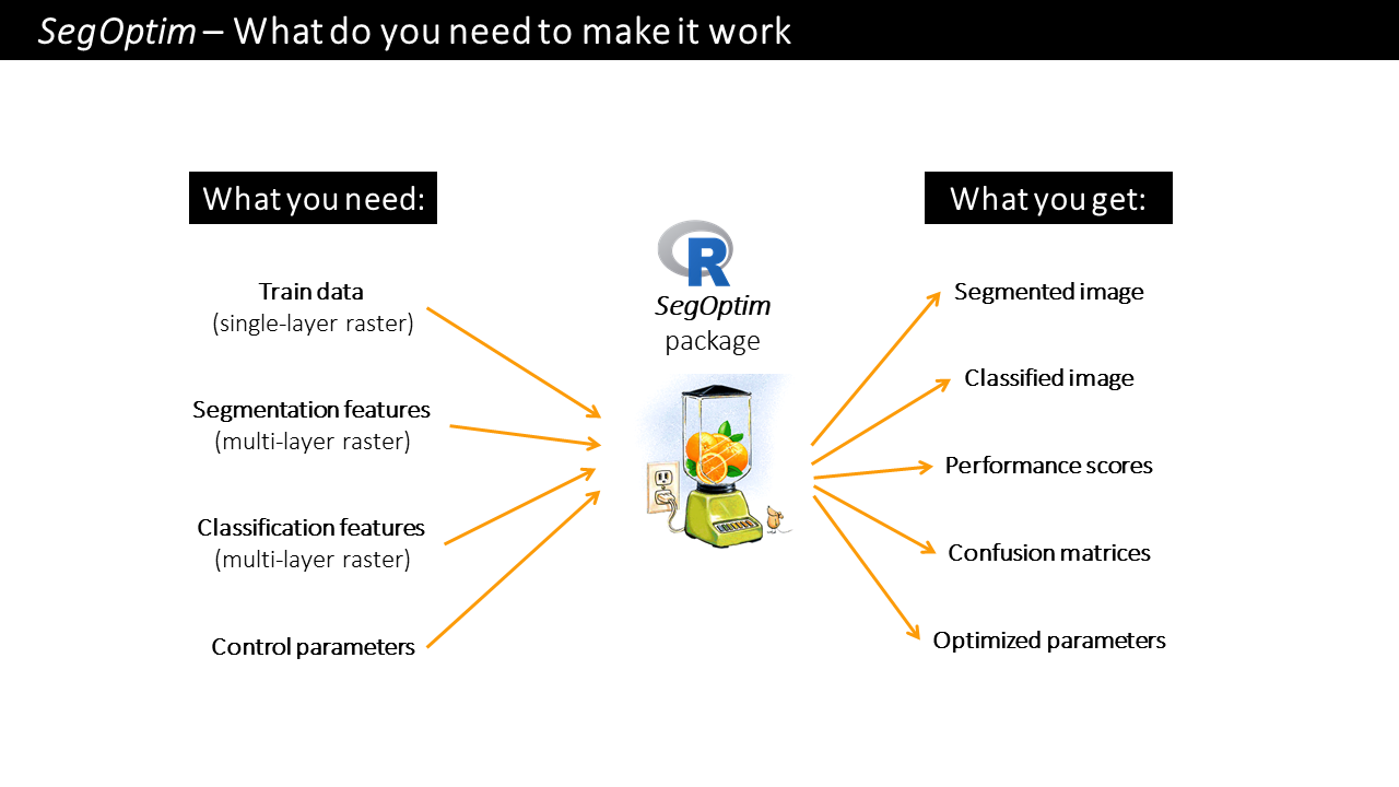
Figure 3.1: SegOptim inputs and outputs

3.3.1 Training data

As mentioned above, training data contains labelled user-provided samples that can be collected through field surveys, digitized based on ancillary data (e.g., satellite or aerial images, previous land cover maps) among other sources and methods.
Ideally, the collection of training data should follow a pre-determined spatial sampling design helping to cover the variability of spectral (or other) characteristics in each class. Another important aspect is the ability of training data to correctly capture the prevalence (i.e., the proportional coverage) of each class in the target area. If some class(es) are disproportionately represented in the training data that will potentially cause problems for classification algorithms. Although relevant, these aspects lay outside the scope of this tutorial. The book by Köhl, Magnussen, and Marchetti (2006) covers most topics in this regard but there many other good reference manuals out there.

How can I create training data to use on SegOptim?

For collecting or digitizing these samples you can start by creating a vector layer (either point or polygon) and proceed to delineate each training point or area. If you are using a polygon layer to collect samples, take into consideration that you should try to completely digitize areas that form relatively homogeneous patches. It is not recommended to digitize partial or not fully-representative areas. However, this may depend on the ancillary data used for this task (namely the spatial resolution).

You can use a software such as QGIS to digitize training data, following a similar workflow:

Start by importing your ancillary image data to the program;
Go to Layer > Create Layer > New Shapefile Layer > Type (Point/Polygon);
Define the field(s) for inputting the class or label for each training point or polygon;
Activate the Digitizing Toolbar and the Advanced Digitizing Panel;
In the toolbar press Toggle Editing and Add features to start collecting training samples.

QGIS manual on vector editing can be found in the following link.

For ArcGIS Desktop the procedure to digitize training samples in vector format is somewhat similar:

Open ArcMap and start by adding all the ancillary data required for digitization;
Go to the ArcCatalog pan, and in a folder location, use the mouse right-button to access options; go to New > Shapefile; 2.1) Set the name of the layer, select the type (point/polygon) and set the coordinate system;
Open the newly created layer in ArcGIS Desktop (if not yet opened);
Add a text or integer field used to label each training point or polygon: Open Attribute Table > Table Options > Add Field...;
Add the Editor toolbar to the interface;
Activate the advanced tools at Editor > More Editing Tools > Advanced Editing and Editor > Editing Windows > Create Features
In the Editor toolbar go to Start Editing and select the layer;
In Construction Tools select Polygon or Point and start adding training instances;
Keep the attribute table opened so you can insert/edit the class label of each instance.

More information regarding the creation of vector maps in ArcGIS can be found here, here, or here.

NOTE!
If you are using polygon training data, you must convert it to raster format before proceeding to classification. The ‘rasterization’ procedure should generate a raster layer with exactly the same extent, number of columns/lines and coordinate reference system as raster inputs used for segmentation.

How is training data incorporated into image segments?

Input training data is a SpatRaster object (from terra package):

In this case, SegOptim uses a simple threshold rule for performing the conversion of user-defined training examples or areas into training segments. This uses a threshold value (\(t=]0,1]\)) defined by the user and the areal proportion (\(a_c\)) of the segment covered by each class \(c=\{0,1\}\) (plus the background or NoData class). Then, the following rule is applied for single-class problems:

\[ \begin{cases} 1,& \text{if } a_{c=1}\geqslant t\\ 0,& \text{otherwise} \end{cases} \] For multi-class problems this threshold rule operates in a slightly different manner. First, a cross-tabulation matrix is generated by calculating the proportion of each segment covered by each land cover class:

Table 3.1: Cross-tabulation by segment and land cover class (SID: segment unique identifier)
SID	Class_1	Class_2	Class_3	…	Class_n	Majority_class
1	0.2	0.8	0.0	…	0.0	2
2	0.5	0.2	0.1	…	0.2	1
3	0.2	0.2	0.2	…	0.4	n
…	…	…	…	…	…	…
N	0.0	0.0	1.0	…	0.0	3

After determining the majority class (i.e., the class with higher areal coverage) the train function
verifies if that class coverage is above or equal to \(t\), otherwise it is removed from the training set. In the example, if \(t=0.5\), then \(SID=\{1,2,N\}\) would be kept while \(SID=\{3\}\) would be removed.

Overall, the higher the value of the threshold \(t\), the ‘purer’ the training segments will be. Hence, this value should reflect the degree to which ‘class-mixing’ at segment-level is allowed for classification.

Input training data is a SpatialPointsDataFrame object:

NOTE!
As of Segoptim’s version 0.3.0, the option to use points as training data has been removed.

3.3.2 Segmentation features

Usually a SpatRaster with multiple layers/bands that can be used to perform the image segmentation step.

Image segmentation can be briefly defined as a process aimed at partitioning an image into multiple segments or regions that are homogeneous according to certain criteria – a process which can employ a variety of image features. For algorithms like mean region growing, Baatz multiresolution, and mean shift segmentation, the selection of features is crucial for effective segmentation.

Often the primary features used in segmentation refer to the different spectral bands (e.g., RGB, near-infrared) and spectral indices. In algorithms like mean region growing, the mean spectral value within a region is often a key criterion for determining whether neighboring pixels or regions should be merged. For images where color is available (e.g., aerial RGB images), color features play a significant role in segmentation. These features are especially important in mean shift segmentation, which analyzes the color space to find dense regions corresponding to different segments.

3.3.3 Classification features

Usually a SpatRaster with multiple layers/bands that can be used to perform the image classification step(s).

Image features used to train machine learning models available in the SegOptim package can come from different sources, such as:

Spectral features: features derived from the various wavelengths/bands captured by satellite sensors. These include the ‘raw’ reflectance values across different bands, such as visible light, red-edge, near-infrared, and thermal infrared. These spectral features can also include band ratios and spectral indices calculated from band combinations.
Spatial/textural features: these features include the texture and structure within the image and can be extracted using techniques like focal analysis (using different kernel sizes), edge detection, gray-level co-occurrence matrix (GLCM), and morphological operations. Spatial features help in distinguishing patterns and structures, like the regular geometric shapes of urban areas versus the more irregular patterns of natural landscapes.
Temporal features: These are particularly relevant in land cover and land use classification. Changes over time can be indicative of certain land uses. For instance, agricultural fields may show seasonal changes corresponding to planting and harvesting cycles. Evergreen and deciduous forest also show very contrasting patterns throughout the year. Satellite time series can capture these dynamic changes.
Contextual or ancillary features: while not direct image features, contextual information such as elevation, slope, terrain geoform from digital elevation models (DEMs) or proximity to known features (like water bodies or urban centers) can significantly enhance classification models.

3.4 Image segmentation

The following sub-sections provide examples of how to use the available image segmentation algorithms. Each algorithm currently interfaced by SegOptim works in widely different ways and require setting different control parameters. However, describing each algorithm and parameter is outside the scope of this tutorial. We refer the user to the SegOptim manual as well as the specific support pages and articles detailing each individual method.

ArcGIS Desktop

Here is a code example for running ArcGIS Mean-shift image segmentation:

# Check the manual for more info on this function parameters
?segmentation_ArcGIS_MShift

segmObj <- segmentation_ArcGIS_MShift(inputRstPath = "C:/DATA/", 
                                     outputSegmRst = NULL, 
                                     SpectralDetail = NULL, 
                                     SpatialDetail = NULL, 
                                     MinSegmentSize = NULL, 
                                     pythonPath = NULL, 
                                     verbose = TRUE)

# Check out the result
rstSegm <- rast(segmObj$segm)

print(rstSegm)
plot(rstSegm)

GRASS GIS

# Check the manual for more info on this function parameters
?segmentation_GRASS_RG

segmObj <- segmentation_GRASS_RG(GRASS.path="grass", 
                                GRASS.inputRstName, 
                                GRASS.GISDBASE, 
                                GRASS.LOCATION_NAME="demolocation",
                                GRASS.MAPSET="PERMANENT", 
                                outputSegmRst=NULL, 
                                Threshold=NULL, 
                                MinSize=NULL, 
                                memory=1024, 
                                iterations=20,
                                verbose=TRUE)

# Check out the result
rstSegm <- rast(segmObj$segm)

print(rstSegm)
plot(rstSegm)

Orfeo ToolBox (OTB)

# Check the manual for more info on this function parameters
?segmentation_OTB_LSMS

segmObj <- segmentation_OTB_LSMS(inputRstPath, 
                                outputSegmRst=NULL, 
                                SpectralRange=NULL, 
                                SpatialRange=NULL, 
                                MinSize=NULL, 
                                lsms_maxiter=10, 
                                tilesizex = 1250, 
                                tilesizey = 1250, 
                                otbBinPath=NULL, 
                                verbose=TRUE)

# Check out the result
rstSegm <- rast(segmObj$segm)

print(rstSegm)
plot(rstSegm)

RSGISLib

# Check the manual for more info on this function parameters
?segmentation_RSGISLib_Shep

segmObj <- segmentation_RSGISLib_Shep(inputRstPath, 
                                      outputSegmRst=NULL, 
                                      NumClust=NULL, 
                                      MinSize=NULL, 
                                      SpectralThresh=NULL, 
                                      pythonPath=NULL, 
                                      verbose=TRUE)

# Check out the result
rstSegm <- rast(segmObj$segm)

print(rstSegm)
plot(rstSegm)

SAGA GIS

# Check the manual for more info on this function parameters
?segmentation_SAGA_SRG

segmObj <- segmentation_SAGA_SRG(rstList, 
                                 outputSegmRst=NULL, 
                                 Bandwidth=NULL, 
                                 GaussianWeightingBW=NULL, 
                                 VarFeatSpace=NULL, 
                                 VarPosSpace=NULL, 
                                 seedType=0, 
                                 method1=0, 
                                 DWeighting=3, 
                                 normalize=0, 
                                 neighbour=0, 
                                 method2=0, 
                                 thresh=0, 
                                 leafSize=1024, 
                                 SAGApath=NULL, 
                                 verbose=TRUE)

# Check out the result
rstSegm <- rast(segmObj$segm)

print(rstSegm)
plot(rstSegm)

INFO
You probably noticed in the manual pages that every function used for image segmentation has a parameter named x (a numeric vector). This parameter is utilized for ‘injecting’ new values (for pre-defined parameters) during optimization and as a result, x is not intended to be directly used. Preferably, for clarity sake, the named parameters should be employed for running the segmentation functions.

3.5 Classification and evaluation

Preparing data for classification

prepareCalData(rstSegm, trainData, rstFeatures, thresh = 0.5, 
                           funs = c("mean","sd"), minImgSegm = 30, verbose = TRUE)

Calibrating the classifier


calibrateClassifier(calData,
                    classificationMethod = "RF",
                    classificationMethodParams = NULL,
                    balanceTrainData = FALSE,
                    balanceMethod = "ubOver",
                    evalMethod = "HOCV",
                    evalMetric = "Kappa",
                    trainPerc = 0.8,
                    nRounds = 20,
                    minTrainCases = 30,
                    minCasesByClassTrain = 10,
                    minCasesByClassTest = 10,
                    runFullCalibration = FALSE)

Classification performance metrics


evalPerf <- evalPerformanceClassifier(obj)

print(evalPerf)

Predicting class labels for the entire image

predictSegments(classifierObj, calData, rstSegm, predictFor = "train", 
                filename=NULL, verbose=TRUE, na.rm=TRUE,...)

References

Köhl, M, S Magnussen, and M Marchetti. 2006. Sampling Methods, Remote Sensing and GIS Multiresource Forest Inventory. 1st Ed. Springer.

SID	Class_1	Class_2	Class_3	…	Class_n	Majority_class
1	0.2	0.8	0.0	…	0.0	2
2	0.5	0.2	0.1	…	0.2	1
3	0.2	0.2	0.2	…	0.4	n
…	…	…	…	…	…	…
N	0.0	0.0	1.0	…	0.0	3

SID	Class_1	Class_2	Class_3	…	Class_n	Majority_class
1	0.2	0.8	0.0	…	0.0	2
2	0.5	0.2	0.1	…	0.2	1
3	0.2	0.2	0.2	…	0.4	n
…	…	…	…	…	…	…
N	0.0	0.0	1.0	…	0.0	3

SID	Class_1	Class_2	Class_3	…	Class_n	Majority_class
1	0.2	0.8	0.0	…	0.0	2
2	0.5	0.2	0.1	…	0.2	1
3	0.2	0.2	0.2	…	0.4	n
…	…	…	…	…	…	…
N	0.0	0.0	1.0	…	0.0	3